Google Satellite Maps Downloader 6.972

© ESO, 2017

1. Introduction

In the standard cosmological framework, the so-called Λ cold dark matter (ΛCDM) paradigm, galaxies form, evolve and reside in dark matter haloes that grow and assemble in a hierarchical way (White & Rees 1978). Therefore, it is assumed that the intrinsic properties and the evolution of these host haloes will have an impact in the subsequent galaxy population inhabiting the haloes. The unknown nature of the dark matter (and dark energy) could be unveiled through the study of the baryonic observables (such as galaxies) once we properly understand their co-evolution, and this task, modelling the relation between the observed galaxy distribution and the underlying dark matter field, is a fundamental question of modern cosmology.

Given a cosmology, the halo mass function, the halo concentration and halo bias can be defined. This implies that the dark matter density field is not perfectly mapped by the distribution of the dark matter haloes, since they are biased tracers of it. In order to model the galaxy clustering statistics, it is necessary to specify the number and spatial distribution of galaxies within these dark matter haloes. One simple approach is to use the statistical halo distribution, known as the standard halo occupation distribution (HOD; Jing et al. 1998; Benson et al. 2000; Seljak 2000; Scoccimarro et al. 2001; Cooray & Sheth 2002; Berlind & Weinberg 2002). Its simplicity resides in the common assumption that the derived occupation parameters and the physical properties of the galaxies are solely determined by the mass of the halo in which they reside. Therefore, the probability that a halo of mass m hosts N_gal galaxies of a given property is given by the quantity P(N_gal | m).

The HOD has been proven a very powerful theoretical tool to constrain both the galaxy-halo connection and the fundamental parameters in cosmology (Yang et al. 2003; Zehavi et al. 2005, 2011; Cooray 2006; van den Bosch et al. 2007; Zheng et al. 2007; Tinker et al. 2013). Through the use of the HOD model, mock galaxy catalogues are constructed for studies of galaxy formation as well as for the preparation and analysis of observational surveys (Berlind & Weinberg 2002; Zheng et al. 2007; Rodríguez-Torres et al. 2016; Carretero et al. 2015). It has become clear, however, that the clustering of dark matter haloes depends on other properties besides mass (Sheth & Tormen 2004; Gao et al. 2005; Conroy et al. 2006; Gao & White 2007; Jing et al. 2007; Wetzel et al. 2007; Faltenbacher & White 2010; Lacerna & Padilla 2011; Lacerna et al. 2014; Pujol & Gaztañaga 2014). For example, the construction of mock galaxy catalogues through N-body simulations hasshown that the amplitude of the two-point correlation function of dark matter haloes with masses lower than 10¹³h^-1M_⊙ on large scales depends on the halo formation time (e.g., Gao et al. 2005). Additionally, halo properties such as concentration, shape, halo spin, major merger rate, triaxiality, shape of the velocity ellipsoid and velocity anisotropy, show correlations with properties other than halo mass (Bett et al. 2007; Croton et al. 2007; Lacerna & Padilla 2012). Moreover, haloes of equal mass could have different galaxy occupation statistics depending on their environment (e.g., Croft et al. 2012; Pujol & Gaztañaga 2014). Ignoring the effects of properties other than mass in the HOD modelling could distort the conclusions and interpretations of the observational results (Zentner et al. 2014).

To solve this issue, new studies point in the direction of taking into account these halo properties linked with the environment and their formation history and modifying the standard HOD accordingly. The relevant properties can be incorporated into the formulation of more flexible schemes of HOD used to produce mock catalogues comparable with observations. Such catalogues have recently been presented by Croton et al. (2007) and Masaki et al. (2013), who introduced a rank ordering of galaxy colours or star formation rate (SFR). The authors point out that, for fixed halo mass, red galaxies are more clustered than blue galaxies. These, together with the “age-matching” models of Hearin et al. (2013, 2014), have been shown to successfully reproduce a number of observed signals such as the two-point clustering and galaxy-galaxy lensing signal of SDSS galaxies (Lacerna et al. 2014, and references therein). Recently, Hearin et al. (2016) presented the idea of decorated HOD, a new parametrisation that allows the galaxy sample to be affected by a parametrised assembly bias.

According to the peak-background split model (Bardeen et al. 1986; Cole & Kaiser 1989), the fundamental quantity that describes halo bias is the density fluctuation of the dark matter field, and not mass. Hence, we expect local density to constrain bias better than mass. In this paper we show the dependence of large scale halo bias on mass and local density (defined as the fluctuations of the local background density ), and confirm the peak-background split prediction that density is the property that constrains bias.

The aim of our study is to analyse how well mass and local density determine galaxy bias and HOD. For this, we present a bias reconstruction method that tests how well the standard HOD assumptions (that halo bias and occupation depend only on mass) are able to correctly predict galaxy bias. To do this, we compare the measured galaxy bias with the one reconstructed from the measurements of halo bias and HOD. This method has already been implemented in Pujol & Gaztañaga (2014), where we showed this test for luminosity dependent galaxy bias. In this paper, we also use the reconstruction method to test how well local density is able to predict galaxy bias from halo bias and HOD. We find that mass is not able to predict galaxy bias for colour-selected samples and that, in these cases, local density makes a much better prediction.

Our analysis is based on haloes from the Millennium simulation (Springel et al. 2005) and the semi-analytical model (SAM) of galaxy formation of Guo et al. (2011). The SAM populate haloes with galaxies that are evolved and followed in time inside the complex structure of merger-trees. The baryonic processes included are laws for metal-dependent gas cooling, reionization, star formation, gas accretion, merging, disk instabilities, AGN and supernovae feedback, ram pressure stripping and dust extinction, among others (e.g., Baugh 2006; Jiménez et al. 2011; Gargiulo et al. 2015). Because of these processes, the resulting galaxy population produced by SAMs is sensitive to the environment and evolution of dark matter haloes. Depending on the galaxy selection, the information from halo mass alone could be insufficiently correlated with the clustering of galaxies. In these cases, local density is more useful for the determination of galaxy bias than halo mass. Thus, we propose to use the information from local density to improve the HOD analyses on surveys and theory.

The paper is organised as follows. In Sect. 2 we describe the data used and the methodology for our measurements of clustering, bias and for our HOD reconstructions. The results are shown in Sect. 3, and we summarise the conclusions of the paper in Sect. 4.

2. Methodology

2.1. Simulation data

In this study we use the data from the Millennium simulation¹ (Springel et al. 2005), an N-body simulation generated using the GADGET-2 code (Springel 2005). The simulation corresponds to a Λ-CDM cosmology with the following parameters: Ω_m = 0.25, Ω_b = 0.045, h = 0.73, Ω_Λ = 0.75, n = 1 and σ₈ = 0.9. It contains 2160³ particles in a comoving box with a side length of 500 h^-1 Mpc. The resolution corresponds to a particle mass of 8.6 × 10⁸h^-1M_⊙ and a spatial resolution of 5 h^-1 kpc. The cosmological model is based on WMAP-1 (Spergel et al. 2003) and the 2-degree Fields Galaxy Redshift Survey (2dFGRS) data (Cole et al. 2005). The initial conditions were calculated using CMBFAST (Seljak & Zaldarriaga 1996). We use the comoving output at z = 0.

The haloes are identified using the friends-of-friends (FOF) algorithm, using a linking length of 0.2 times the mean particle separation, and discarding all haloes with less than 20 particles. In our analysis we define the halo mass from the total number of particles belonging to the FOFs.

Galaxy catalogues of several SAM are available in the public database of the simulation. For this analysis we used four models (Bower et al. 2006; De Lucia & Blaizot 2007; Font et al. 2008; Guo et al. 2011). Although the results are different for each model, they all show the same behaviours and the conclusions of our study do not depend on the SAM used. For this, we show the results from Guo et al. (2011) in Sect. 3, and we show a comparison of the rest of the models in Appendix A.

2.2. Clustering and bias

Spatial fluctuations of the matter or tracer density ρ are defined as normalised deviations from the mean density at the position r, that is, (1)Note that in this article we often refer to these density fluctuations as density for simplicity. We measure δ(r) by dividing the simulation into cubical grid cells with side lengths of 500/64 ~ 8 h^-1 Mpc and assigning a δ to each cell. We then measure the two-point correlation function as (2)which is a function of the scale r ≡ | r₂−r₁ |. The average ⟨ ... ⟩ is taken over all pairs of δ in the analysed volume, independently of their orientation. The indices A and B refer to the fluctuations of different density tracers (here haloes or galaxies, which we generically call δ_G) or to those of the matter density, which we denote as δ_m. Hence, A = B = m denotes the matter auto-correlation (ξ_mm), while ξ_Gm is the cross-correlation between the tracer G and matter m. We then estimate the bias by the ratio: (3)At large scales (r ≳ 20 h^-1 Mpc), where ξ< 1, this ratio is well described by a constant, which is in good agreement with the linear bias and tends to the value δ_G ≃ b₁δ_m, (e.g. see Bel et al. 2015). We estimate this linear bias b₁, which we refer to as b, by fitting b(r) with a constant in the scale range of 20 h^-1 Mpc <r< 30 h^-1 Mpc. For larger scales, the measurements start to be noisy due to the size of the simulation. The covariance of these measurements is derived by jack-knifing (e.g. Norberg et al. 2009) using 64 cubical subvolumes.

The value of b depends on how the tracers are selected. In galaxy surveys, the limits of the observed galaxy luminosities roughly correspond to a selection by host halo mass. The mass dependence of the bias can be predicted from the peak-backgroundsplit model (see Bardeen et al. 1986; Cole & Kaiser 1989; Mo & White 1996; and Hoffmann et al. 2015, for a recent validation of the predictions) where the matter density field is described by the superposition of small-scale fluctuations (peaks) δ_s with large-scale fluctuations of the background matter density around each peak (i.e. ). In this model background fluctuations can lift the peak-heights above a critical density δ_crit at which they collapse to haloes as illustrated by Fig. 1. The mass of these haloes then corresponds to the peak-heights. Consequently massive haloes tend to reside in environments where the background density is high, while low-mass haloes can reside in a broader range of environmental densities (we show this effect with haloes from the Millennium simulation in Sect. 3.1). Massive haloes are therefore more strongly clustered than low-mass haloes, which causes a mass dependence of the bias parameter.

2.3. Local background density

The bias of a given halo sample can also depend on additional halo properties besides the halo mass, such as the concentration of the mass density profile or the properties of the galaxies hosted by the halo (see e.g. Gao et al. 2005; Faltenbacher & White 2010; Hearin et al. 2015). These additional properties can be related to the merging history of haloes and lead to the so-called assembly bias. Furthermore, the bias of a given halo sample is affected by the tidal forces from the large-scale environment, which is known as non-local bias (see Chan et al. 2012; Baldauf et al. 2012; Bel et al. 2015).

	Fig. 1 Illustration of peak-background split model, , showing the location of haloes that form above some critical value δcrit in red. The clustering of those haloes is stronger than the rest (in green). But note how once the local density (black curve) is fixed at δcrit, the large-scale clustering of haloes (red) does not depend on the peak-hight (halo mass).
Open with DEXTER

These effects can lead to false predictions by models that rely on the assumption that the mass of a halo sample completely determines the bias, such as self-calibration techniques (e.g. Wu et al. 2008) or HOD models (Zentner et al. 2014; Pujol & Gaztañaga 2014). A way to circumvent problems for the HOD model is to use a halo property different from the mass, which completely determines the bias of a given halo population. The peak-background split argument described in Sect. 2.2 suggests that the clustering of peaks (which corresponds to tracers such as haloes) is determined by fluctuations of the large-scale background density . Hence, for fixed background densities, the bias should be independent of the tracer properties (see Fig. 1 for illustration).

To obtain a visual impression of this argument, in Fig. 2 we show the spatial distribution of haloes that reside in regions with different densities, defined by the value of estimated around each halo smoothed on cubical cells of side l = 14 h^-1 Mpc as explained below. By comparing the four panels of the figure one can see that the large-scale clustering, and hence the bias, strongly changes with the local dark matter back-ground density (as we show in Sect. 3.2). On the other hand, the large-scale clustering is nearly independent of halo mass (not shown in this figure) when haloes are selected by . Note that a weak mass dependence of the bias for fixed can be expected from the aforementioned non-local bias.

	Fig. 2 Distribution of haloes with different dark matter local densities in a 2 h-1 Mpc slice of the Millennium simulation. The top left panel shows all haloes, while the top right shows haloes in under-densities. The bottom left shows haloes with mean background densities while the bottom right shows haloes in over-dense regions.
Open with DEXTER

When determining around a given halo, we face the problem that the dark matter density distribution of the Millennium simulation is only publicly available as a 500/256 ≃ 2 h^-1 Mpc grid. We therefore assigned the density in a cubical volume around each halo, with length l ≃ 6,14 and 26 h^-1 Mpc, which have the same volume as a sphere of radius R = 3.72,8.68 and 16.13 h^-1 Mpc, respectively. The position of these volumes has a 2 h^-1 Mpc inaccuracy, which results from the grid cell size. In the presentation of our results we focus on the intermediate scale R = 8.68 h^-1 Mpc, while this choice does not affect our conclusion, as results for the other scales are similar.

The linear halo bias b_h is shown as a function of in Fig. 3 using haloes of all masses. The bias increases with the density of the environment and becomes negative in under-dense regions. Note that we find negative bias because we study the halo-matter cross-correlation, while in the case of the auto-correlation the bias would remain positive.The dependence of b_h on becomes weaker when is defined at smaller scales R. Note that the clustering of galaxy with different environmental densities has been studied in data by Abbas & Sheth (2007).

Since the large-scale clustering of the tracers corresponds to the clustering of the background density fluctuations in which they reside, we can compare our measurements to predictions for the clustering of the excursion set model (Sheth 1998). We use Eq. (5) from Abbas & Sheth (2007): (4)where is the initial linear over-density and σ₀ is the corresponding linear variance on the Lagrangian scale . To estimate , we use the spherical collapse model to map the measured non-linear local density into the initial density (see also Fosalba & Gaztanaga 1998). These predictions are in general in good agreement with the measurements and do not include any free parameters. Note that some of the differences at small could come from the fact that we measure the bias in bins of , while the prediction are for threshold values of , so we expect them to be systematically higher. This can easily be corrected, but is beyond the scope of this paper.

In the following subsection we will directly use these bias measurements to study the bias predictions from the standard HOD assumptions, and to present a new HOD test based on local density , which is less affected by assembly bias.

	Fig. 4 Left: halo bias as a function of mass. Each line corresponds to haloes in a fixed density fluctuations . Right: halo bias as a function of the local density . Each line corresponds to a different halo mass bin. In both panels, is defined as the Eulerian density fluctuation around a cubic box of 14 h-1 Mpc of side.
Open with DEXTER

2.4. Mass and density HOD bias reconstruction

The standard HOD model is based on the assumption that halo bias is determined solely by the halo mass m of the sample. We will therefore refer to it as the mHOD model in the following. In this mHOD model, the bias of galaxies (b_g), which are selected by an arbitrary property P, are reconstructed from the halo bias as a function of mass b_h(m) and the mean number of galaxies with property P per halo with mass m, ⟨ N_g(m | P) ⟩ as (5)This equation can be seen as a weighted average of b_h(m), where the weight is given by ⟨ N_g(m | P) ⟩. The mHOD model provides a way to infer the average mass of host haloes in which a given galaxy population is residing by varying ⟨ N_g(m | P) ⟩ in order to reproduce the observed bias, that is, . However, this relies on the assumption that the bias of a galaxy population selected by the property P is completely determined by their host halo mass, which might not be correct as discussed in Sect. 2.2. Cosmological N-body simulations allow us to test the mHOD model, as we can measure b_h(m) and ⟨ N_g(m | P) ⟩ and compare the predicted to measurements of b_g(P). This test was explored by Pujol & Gaztañaga (2014) and will hereafter be referred to as the bias reconstruction method. The test revealed that the mHOD model fails to predict the bias correctly in the low halo mass rangebut that it works with 5–10% bias accuracy in the high mass end.

In the previous subsection we considered the redefinition of the HOD model using the local background density around a given halo instead of the halo mass. This approach has the advantage that is expected to determine the bias of a given halo or galaxy population better than the mass (we study this in Sect. 3). Furthermore, is well defined, whereas the halo mass can vary significantly, depending on the definition. In this paper we refer to the density HOD (dHOD) model (using density), analogous to the mHOD model (using mass). The corresponding bias reconstruction is obtained simply by replacing the halo mass in Eq. (5) by , (6)In the following section we test how well our new dHOD model predicts the bias compared to the standard mHOD model.

3. Results

3.1. Halo bias

In this subsection we analyse the dependence of halo bias on halo mass and local background matter density fluctuations (smoothed with a cubical top hat filter with a side length of l = 14 h^-1 Mpc, which has the same volume as a sphere of radius R = 8.68 h^-1 Mpc) in the environment of each halo. The measurement of the latter is described in Sect. 2. Similar results are found for other smoothing scales.

In the left panel of Fig. 4 we show the halo bias (b_h), measured via Eq. (3), as a function of the halo mass m for haloes within different ranges. The black line corresponds to b_h(m) for all haloes, selected independently of . This latter measurement is consistent with the theoretical model of Tinker et al. (2010; see Fig. 3 of Pujol & Gaztañaga 2014). We can see that b_h(m) does not change significantly (less than a 10%) with halo mass when is fixed, while it changes significantly when all the haloes are included (by approximately a factor of 2 in the range of masses shown here). In the right panel we show the same analysis from a different point of view. Here we present for different m bins. Each line corresponds to a range in m, while the black solid line shows for all the haloes. We can see a strong dependence of b_h on , and that depends weakly on m.

These measurements demonstrate the argument from the peak-background split that local density is the property that constrains clustering. We show that the bias of a given halo sample is well constrained when the haloes are solely selected by the local density in their environment , almost independently of the halo mass.

If is left as a free parameter, a mass dependence of the bias arises from the fact that high mass haloes tend to reside in high density regions and low mass haloes in regions with lower density. This tendency can be seen in the central panel of Fig. 5, where we show the mass versus the local density for each halo in the simulation. The colours describe the number of haloes with the corresponding mass and density. By integrating this distribution over we derive the HMF, (where V is the simulation volume and N_h the absolute number of haloes). The HMF is well described by the Tinker et al. (2008) model, as shown in the top panel of Fig. 5. By integrating over the mass m, we obtain the probability distribution function (PDF) of , or , which is roughly log-normal, as shown in the right panel of Fig. 5.

The aforementioned tendency, that high mass haloes tend to reside in high density regions and low mass in regions with lower density, can be seen more clearly in Fig. 6. In the top panel of this figure we show the HMF of haloes with different background densities . We find that the fraction of massive haloes decreases in low densities, while the fraction of low mass haloes is similar. The same effect can be seen in the bottom panel of this figure, where we show the PDF of for haloes in different mass bins. We find that massive haloes (i.e m> 10¹⁴h^-1M_⊙) reside almost exclusively in very dense regions and are unlikely to be found in regions with low density, while low-mass haloes can be found in a wide range of densities, with preference to average values of .

The dependence of the b_h(m) measurements on the local halo background density is in agreement with Abbas & Sheth (2007). This result is to be expected, since is defined from larger scales than m, and larger scales are expected to better determine bias. The standard HOD model assumes that halo bias is determined solely by the halo mass, but the local density contains additional information that constrains bias. We therefore test the accuracy of mHOD reconstructions in the following subsection and compare it to reconstructions from our new dHOD model from Eq. (6), which is based on the assumption that the bias is determined solely by , as discussed in Sect. 2 and suggested by the results of this subsection.

	Fig. 6 Distributions of haloes in m and . Top panel shows the HMF for haloes in different densities. Each colour represents haloes in a range of . The bottom panel shows the PDF of of haloes of different masses. Different colours represent haloes of different m ranges.
Open with DEXTER

	Fig. 7 Halo bias reconstructions compared to the measured bias from the simulation. The solid black lines show the measurement of bh from the simulation. The coloured regions show the 1σ interval of the reconstructions. The top panel shows (in grey) from bh(m), while the bottom panel shows (in red) from .
Open with DEXTER

3.2. HOD tests using mass and density

In this subsection we study how well mass m and local density determine the linear bias of a given halo sample. We do this by testing how well the mHOD model can predict the halo bias as a function of background density and how well the dHOD model can predict the halo bias as a function of halo mass m. The reconstruction for from the mHOD model is derived by averaging the b_h(m) measurement using the measured as weight, as given by Eq. (5). This reconstruction is then compared with measurements of , derived from the two-point correlations via Eq. (3). The dHOD reconstructions for b_h(P = m) is tested in an analogous way using and measurements in combination with Eq. (6).

We can see in the top panel of Fig. 6 that the HMF depends on in the high mass end only, while in the low mass end, changes in lead to relatively small fluctuations in HMF. Since the low mass end of the HMF dominates the integral of the mHOD bias reconstruction from Eq. (5), we do not expect to be strongly dependent on . The PDF of in the bottom panel of Fig. 6 shows that haloes of different m are differently distributed in . Therefore we expect a strong dependence of from Eq. (6) on m.

The bias reconstructions and are compared with the measured bias and b_h(m) in Fig. 7. As expected from our considerations above, the reconstruction does not show a significant dependence and therefore it deviates from the measured . This finding means that, once is fixed, the halo mass (or peak height) does not contain additional information about the large-clustering, which already became apparent in the weak mass dependence of the bias of haloes with fixed , shown in Fig. 4. Hence, the clustering of a given halo sample selected by cannot be reconstructed via the standard mHOD model.

The b_h(m) dHOD reconstruction, , shown in the bottom panel of Fig. 7, is in much better agreement with the measurement. This finding demonstrates that the bias is accurately determined by . The over prediction of b_h by the dHOD model at high halo masses results from the fact that b_h is not completely independent of the mass at fixed , as we see in the left panel of Fig. 4.

3.3. HOD modelling of galaxy bias

The results presented in the previous subsection confirm the peak-background split model and have important implications on HOD modelling of galaxy clustering as galaxy properties are not only determined by the mass of their host halo, but also by their interaction with the environment.

Assuming that bias solely depends on the halo mass can lead to a misinterpretation of HOD predictions (e.g. the fraction of red satellites) and false predictions of galaxy bias as a function of galaxy properties, such as colour or luminosity (Pujol & Gaztañaga 2014; Zentner et al. 2014). In these cases, it can be worthwhile to use the local density for HOD bias predictions, since we have shown that it determines the bias better than halo mass.

In Fig. 8 we show the comparison of the different HOD reconstruction methods in two different samples of central galaxies from the Guo et al. (2011) SAM. In this analysis we focus on central galaxies, since their properties are more correlated with the halo properties than satellite or orphans galaxies, and the implications of the local density dependence of halo bias are more directly connected to this population.

The top panel shows the bias of central galaxies as a function of the colour index g−r = M_g−M_r, where M_g and M_r are the absolute magnitudes in the SDSS g- and r-band, taking into account dust extinction. The bias values below unity result from the fact that we did not apply a faint magnitude cut to the samples. They are therefore dominated by dim galaxies with low clustering. The bottom panel shows the bias of red central galaxies (g−r> 0.6) versus M_r. The solid black line shows the galaxy bias b_g measured from the two-point correlation via Eq. (3). The grey regions show the 1σ interval of the mHOD reconstruction for b_g from Eq. (5), that indicates how well m determines bias for these galaxy samples. The red regions show the 1σ interval of the dHOD reconstruction of b_g from Eq. (6), that reflects how well determines bias for these galaxies.

We can clearly see that the dHOD reconstruction is much closer to the measured bias than reconstruction from the mHOD model. This finding indicates that determines b_g much better than m. This is related to the formation times of the haloes and their assembly history. In terms of galaxy formation, SAMs show that galaxy colours are affected by merging events (Jiménez et al. 2011, and references therein) which occur more often in high density environments. We conclude that, when galaxy properties are determined by halo local density, the standard mHOD model can fail to predict the bias as a function of that property. In this case, HOD bias predictions based on the more fundamental halo property , that is, the dHOD model, deliver more accurate bias predictions. This effect is not always as important as in Fig. 8, as we can see from Pujol & Gaztañaga (2014). In this work, b_g is shown as a function of absolute magnitude, and since magnitude and mass are well related for these galaxies, the mHOD reconstruction works well.

In real galaxy catalogues it is very difficult to measure the mean matter density, , that we are using to define environment. Instead we can easily measure , the density fluctuations of galaxies. In Fig. 8 we also show the bias reconstruction using instead of , (), represented as blue regions. We measure from galaxies of M_r< −19, and clearly see that the result is equivalent to that using ; in fact it is even better. This means that determines bias in a similar way to, or better than, . This result is to be expected as large scale fluctuations in and are simply related to each other by the linear bias of the background galaxy sample. Also note that is more closely related to the galaxy distribution than (the relation between and might have stochasticity, for example) so it is not surprising that gives a slightly better reconstruction than . It is important to mention that different galaxy formation models generally present different galaxy distributions. Because of this, the relation between galaxy bias and halo mass or local density can be different depending on the implemented galaxy formation model. For galaxy formation models based on the HOD, constructed using only the halo mass to define the galaxy populations, we would expect, by construction, a better agreement between b_g and . However, these HOD models would be then totally insensitive to assembly bias effects. This is not the case for SAMs, since these models are constructed from the halo merger trees. This study has been done using four different SAMs in order to see how much our conclusions depend on different implementations of SAMs. We have seen that all SAMs present the same behaviour, and we show the comparison of these models in Appendix A.

4. Conclusions

In this paper we use the Millennium simulation (Springel et al. 2005) and their public catalogues to study the impact of halo mass and local density on the prediction of linear bias.

We study the dependence of halo bias on mass (FOF mass) and local density, defined as the density fluctuation within a given volume around each halo. Although for this paper we used a cubical box of side l = 14 h^-1 Mpc (which has the same volume as a sphere of radius R = 8.68 h^-1 Mpc), we verified that the results are similar if we use other scales. We also find similar results when we use Lagrangian instead of Eulerian densities for the background.

We show that bias depends much more strongly on than on mass, and once is fixed, the halo bias depends very weakly on mass. This is important, since it reflects the fact that the halo bias is well constrained when the haloes are selected by the local density, almost independently from the mass. More massive haloes have a higher clustering because, statistically, they are in denser regions, but not because mass is the fundamental cause of clustering. In particular, low-mass haloes can be found in a wide range of densities, and hence these haloes present different clustering. These results confirm the peak-background split model, that states that the large-scale clustering is determined by the density fluctuations of matter, and not by halo mass. This is in contradiction with the standard HOD implementation which assumes that halo bias only depends on the mass. The local density can be seen as a property that is sensitive to other dependencies of halo bias apart from mass, such as assembly bias. Assembly bias usually refers to the difference in clustering from haloes of equal mass but different formation time or concentration. These differences can indeed be related to the local density, as haloes in high background densities form first and have higher concentrations. This can also explain the concept of galactic conformity (see Paranjape et al. 2015, and references therein) by which galaxy properties, such as luminosity and colour, are not solely determined by the mass of the halo. Thus, our finding that halo local density, and not halo mass, is the key variable in understanding the large-scale clustering of haloes is in line with these previous results.

To study the implication of our finding for the clustering predictions in the HOD framework, we use the method of reconstructing the linear bias from the halo bias and the occupation distribution in haloes, as explained in Pujol & Gaztañaga (2014) and in this paper. This can be seen as a test of how well mass and local density constrain bias. More precisely, these bias reconstructions measure how well linear bias can be reproduced by assuming that the halo bias and occupation only depend on one variable (either mass or density around the halo). We show that we can predict b_h(M) from , but we cannot predict from b_h(M). This means that determines bias better than M. This is important for HOD analysis, since it is usually assumed that bias only depends on halo mass, but some galaxy populations might be affected by environment and local density as well. According to our results, the dependencies of galaxies on the environmental density have a stronger impact on the large scale clustering than the dependencies on halo mass. With the exception of the higher mass range, which is strongly correlated with background density, as shown in Fig. 5, and therefore shows similar tendencies than local density.

Some of the galaxy properties can be sensitive to assembly bias and the local density. In these cases, assuming that linear bias only depends on halo mass causes an error in our estimation of clustering or in the estimation of HOD parameters. Instead, we can use the local density as a proxy for bias, since on large scales it determines bias better than mass.

We show two examples of galaxy samples, b(M_r) of red central galaxies and b(g−r) of central galaxies, where the galaxy clustering does not depend only on halo mass. We see that the reconstruction using the local density around the haloes makes a good prediction of galaxy bias, but the standard reconstruction using halo mass does not recover the galaxy bias well. This means, on the one hand, that the occupation of this population of galaxies in haloes is affected by the local density even for fixed mass, and on the other hand, that even if the occupation of these galaxies in haloes depends on mass, the clustering of these galaxies is mainly due to the dependence on the local density. We also used instead of to measure the local density of haloes and the results are equivalent to those using , meaning that both and are good estimators of bias. This result is to be expected, since at large scales, is biased with respect to , but the nature of both properties is the same, and hence they disclose similar information about the local density. The advantage of using is that it can be directly measured in observations, while or halo mass are more difficult to estimate. We also show that our results and conclusions do not depend on the SAM used for the analysis.

This analysis is focused on linear scales, where the 2-halo term dominates, therefore we do not need to assume anything about the distribution of galaxies inside the haloes. A similar analysis is relevant for the 1-halo term, since small scales can also depend on local density. For example, the satellite distribution can depend on the halo concentration for fixed mass. Also, these linear scales now become more accessible with upcoming surveys. As is a better estimator of large-scale clustering than mass, and it is also easier to measure in observations (at large scales is simply a biased version of ), this method can be applied in observations to measure the bias as a function of , and to study galaxy clustering from the modelling of instead of simply b_h(M) in order to incorporate the information from assembly bias and environmental dependencies of bias.

Acknowledgments

Are you in need of uninstalling iPWebCam Central 2.0.0.0 to fix some problems? Are you looking for an effective solution to completely uninstall it and thoroughly delete all of its files out of your PC? No worry! This page provides detailed instructions on how to completely uninstall iPWebCam Central 2.0.0.0.

Possible problems when you uninstall iPWebCam Central 2.0.0.0

* iPWebCam Central 2.0.0.0 is not listed in Programs and Features.
* You do not have sufficient access to uninstall iPWebCam Central 2.0.0.0.
* A file required for this uninstallation to complete could not be run.
* An error has occurred. Not all of the files were successfully uninstalled.
* Another process that is using the file stops iPWebCam Central 2.0.0.0 being uninstalled.
* Files and folders of iPWebCam Central 2.0.0.0 can be found in the hard disk after the uninstallation.

iPWebCam Central 2.0.0.0 cannot be uninstalled due to many other problems. An incomplete uninstallation of iPWebCam Central 2.0.0.0 may also cause many problems. So, it's really important to completely uninstall iPWebCam Central 2.0.0.0 and remove all of its files.

How to Uninstall iPWebCam Central 2.0.0.0 Completley?

Method 1: Uninstall iPWebCam Central 2.0.0.0 via Programs and Features.

When a new piece of program is installed on your system, that program is added to the list in Programs and Features. When you want to uninstall the program, you can go to the Programs and Features to uninstall it. So when you want to uninstall iPWebCam Central 2.0.0.0, the first solution is to uninstall it via Programs and Features.

Steps:

a. Open Programs and Features.

Windows Vista and Windows 7

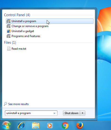
Click Start, type uninstall a program in the Search programs and files box and then click the result.

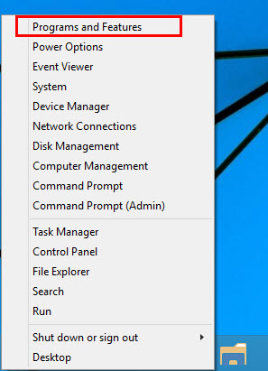
Windows 8, Windows 8.1 and Windows 10

Open WinX menu by holding Windows and X keys together, and then click Programs and Features.

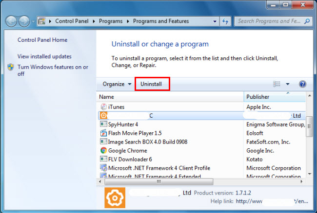
b. Look for iPWebCam Central 2.0.0.0 in the list, click on it and then click Uninstall to initiate the uninstallation.

Method 2: Uninstall iPWebCam Central 2.0.0.0 with its uninstaller.exe.

Most of computer programs have an executable file named uninst000.exe or uninstall.exe or something along these lines. You can find this files in the installation folder of iPWebCam Central 2.0.0.0.

Steps:

a. Go to the installation folder of iPWebCam Central 2.0.0.0.

b. Find uninstall.exe or unins000.exe.

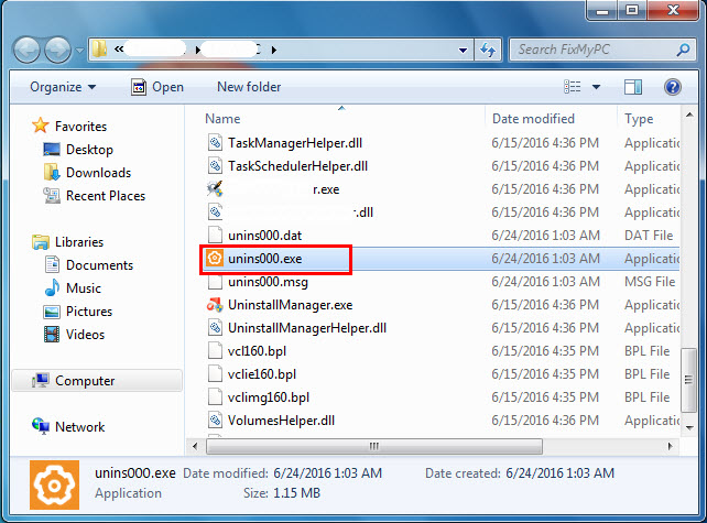
c. Double click on its uninstaller and follow the wizard to uninstall iPWebCam Central 2.0.0.0.

Method 3: Uninstall iPWebCam Central 2.0.0.0 via System Restore.

System Restore is a utility which comes with Windows operating systems and helps computer users restore the system to a previous state and remove programs interfering with the operation of the computer. If you have created a system restore point prior to installing a program, then you can use System Restore to restore your system and completely eradicate the unwanted programs like iPWebCam Central 2.0.0.0. You should backup your personal files and data before doing a System Restore.

Steps:

a. Close all files and programs that are open.

b. On the desktop, right click Computer and select Properties. The system window will display.

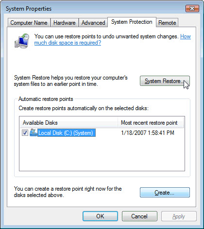
c. On the left side of the System window, click System protection. The System Properties window will display.

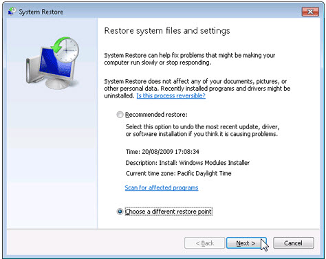
d. Click System Restore and the System Restore window will display.

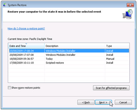
e. Select Choose a different restore point and click Next.

f. Select a date and time from the list and then click Next. You should know that all programs and drivers installed after the selected date and time may not work properly and may need to be re-installed.

g. Click Finish when the "Confirm your restore point" window appears.

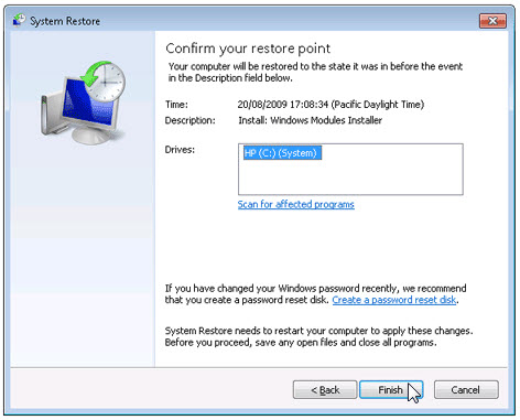
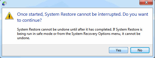
h. Click Yes to confirm again.

Method 4: Uninstall iPWebCam Central 2.0.0.0 with Antivirus.

Nowadays, computer malware appear like common computer applications but they are much more difficult to remove from the computer. Such malware get into the computer with the help of Trojans and spyware. Other computer malware like adware programs or potentially unwanted programs are also very difficult to remove. They usually get installed on your system by bundling with freeware software like video recording, games or PDF convertors. They can easily bypass the detection of the antivirus programs on your system. If you cannot remove iPWebCam Central 2.0.0.0 like other programs, then it's worth checking whether it's a malware or not. Click and download this malware detect tool for a free scan.

Method 5: Reinstall iPWebCam Central 2.0.0.0 to Uninstall.

When the file required to uninstall iPWebCam Central 2.0.0.0 is corrupted or missing, it will not be able to uninstall the program. In such circumstance, reinstalling iPWebCam Central 2.0.0.0 may do the trick. Run the installer either in the original disk or the download file to reinstall the program again. Sometimes, the installer may allow you to repair or uninstall the program as well.

Method 6: Use the Uninstall Command Displayed in the Registry.

When a program is installed on the computer, Windows will save its settings and information in the registry, including the uninstall command to uninstall the program. You can try this method to uninstall iPWebCam Central 2.0.0.0. Please carefully edit the registry, because any mistake there may make your system crash.

Steps:

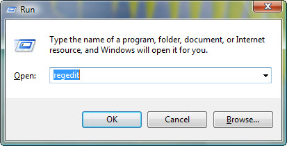
a. Hold Windows and R keys to open the Run command, type in regedit in the box and click OK.

b. Navigate the following registry key and find the one of iPWebCam Central 2.0.0.0:

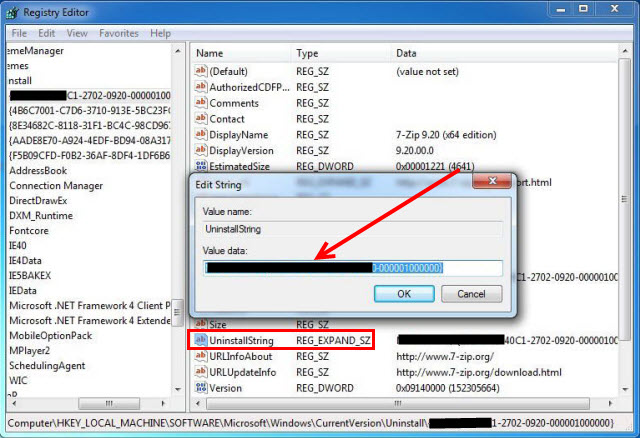
HKEY_LOCAL_MACHINE\SOFTWARE\Microsoft\Windows\CurrentVersion\Uninstall

c. Double click on the UninstallString value, and copy its Value Data.

d. Hold Windows and R keys to open the Run command, paste the Value Data in the box and click OK.

e. Follow the wizard to uninstall iPWebCam Central 2.0.0.0.

Method 7: Uninstall iPWebCam Central 2.0.0.0 with Third-party Uninstaller.

The manual uninstallation of iPWebCam Central 2.0.0.0 requires computer know-how and patience to accomplish. And no one can promise the manual uninstallation will completely uninstall iPWebCam Central 2.0.0.0 and remove all of its files. And an incomplete uninstallation will many useless and invalid items in the registry and affect your computer performance in a bad way. Too many useless files also occupy the free space of your hard disk and slow down your PC speed. So, it's recommended that you uninstall iPWebCam Central 2.0.0.0 with a trusted third-party uninstaller which can scan your system, identify all files of iPWebCam Central 2.0.0.0 and completely remove them. Download this powerful third-party uninstaller below.