
MedCalc 7.6.0.0 serial key or number

MedCalc 7.6.0.0 serial key or number
Performance of ultralow-dose CT with iterative reconstruction in lung cancer screening: limiting radiation exposure to the equivalent of conventional chest X-ray imaging
Abstract
Objective
To investigate the detection rate of pulmonary nodules in ultralow-dose CT acquisitions.
Materials and methods
In this lung phantom study, 232 nodules (115 solid, 117 ground-glass) of different sizes were randomly distributed in a lung phantom in 60 different arrangements. Every arrangement was acquired once with standard radiation dose (100 kVp, 100 references mAs) and once with ultralow radiation dose (80 kVp, 6 mAs). Iterative reconstruction was used with optimized kernels: I30 for ultralow-dose, I70 for standard dose and I50 for CAD. Six radiologists examined the axial 1-mm stack for solid and ground-glass nodules. During a second and third step, three radiologists used maximum intensity projection (MIPs), finally checking with computer-assisted detection (CAD), while the others first used CAD, finally checking with the MIPs.
Results
The detection rate was 95.5 % with standard dose (DLP 126 mGy*cm) and 93.3 % with ultralow-dose (DLP: 9 mGy*cm). The additional use of either MIP reconstructions or CAD software could compensate for this difference. A combination of both MIP reconstructions and CAD software resulted in a maximum detection rate of 97.5 % with ultralow-dose.
Conclusion
Lung cancer screening with ultralow-dose CT using the same radiation dose as a conventional chest X-ray is feasible.
Key points
• 93.3 % of all lung nodules were detected with ultralow-dose CT.
• A sensitivity of 97.5 % is possible with additional image post-processing.
• The radiation dose is comparable to a standard radiography in two planes.
• Lung cancer screening with ultralow-dose CT is feasible.
This is a preview of subscription content, log in to check access.
Abbreviations
Computer-aided detection
Maximum intensity projection
References
- 1.
Jemal A, Bray F, Center MM et al (2011) Global cancer statistics. CA Cancer J Clin 61:69–90
ArticlePubMed Google Scholar
- 2.
Kaneko M, Eguchi K, Ohmatsu H et al (1996) Peripheral lung cancer: screening and detection with low-dose spiral CT versus radiography. Radiology 201:798–802
CASArticlePubMed Google Scholar
- 3.
Henschke CI, Yankelevitz DF, Libby DM et al (2006) Survival of patients with stage I lung cancer detected on CT screening. N Engl J Med 355:1763–1771
ArticlePubMed Google Scholar
- 4.
The National Lung Screening Trial Team (2011) Reduced lung-cancer mortality with low-dose computed tomographic screening. N Engl J Med 365:395–409
Article Google Scholar
- 5.
Field JK, van Klaveren R, Pedersen JH et al (2013) European randomized lung cancer screening trials: post NLST. J Surg Oncol 108:280–286
ArticlePubMed Google Scholar
- 6.
van Iersel CA, de Koning HJ, Draisma G et al (2007) Risk-based selection from the general population in a screening trial: selection criteria, recruitment and power for the Dutch-Belgian randomised lung cancer multi-slice CT screening trial (NELSON). Int J Cancer 120:868–874
ArticlePubMed Google Scholar
- 7.
Wender R, Fontham ETH, Barrera E et al (2013) American cancer society lung cancer screening guidelines. CA Cancer J Clin 63:106–117
Article Google Scholar
- 8.
Jaklitsch MT, Jacobson FL, Austin JHM et al (2012) The American association for thoracic surgery guidelines for lung cancer screening using low-dose computed tomography scans for lung cancer survivors and other high-risk groups. J Thorac Cardiovasc Surg 144:33–38
ArticlePubMed Google Scholar
- 9.
Nair A, Hansell DM (2011) European and North American lung cancer screening experience and implications for pulmonary nodule management. Eur Radiol 21:2445–2454
ArticlePubMed Google Scholar
- 10.
Kauczor H-U, Bonomo L, Gaga M, et al. (2015) ESR/ERS white paper on lung cancer screening. Eur Respir J ERJ–00330–2015. doi: 10.1183/09031936.00033015
- 11.
Mahadevia PJ, Fleisher LA, Frick KD et al (2003) Lung cancer screening with helical computed tomography in older adult smokers: a decision and cost-effectiveness analysis. JAMA J Am Med Assoc 289:313–322
Article Google Scholar
- 12.
Swensen SJ, Jett JR, Sloan JA et al (2002) Screening for lung cancer with low-dose spiral computed tomography. Am J Respir Crit Care Med 165:508–513
ArticlePubMed Google Scholar
- 13.
Brenner DJ (2004) Radiation risks potentially associated with low-dose CT screening of adult smokers for lung cancer. Radiology 231:440–445
ArticlePubMed Google Scholar
- 14.
Baumueller S, Winklehner A, Karlo C et al (2012) Low-dose CT of the lung: potential value of iterative reconstructions. Eur Radiol 22:2597–2606
ArticlePubMed Google Scholar
- 15.
Neroladaki A, Botsikas D, Boudabbous S et al (2013) Computed tomography of the chest with model-based iterative reconstruction using a radiation exposure similar to chest X-ray examination: preliminary observations. Eur Radiol 23:360–366
ArticlePubMed Google Scholar
- 16.
Gordic S, Morsbach F, Schmidt B et al (2014) Ultralow-Dose chest computed tomography for pulmonary nodule detection: first performance evaluation of single energy scanning with spectral shaping. Invest Radiol 49:465–473
ArticlePubMed Google Scholar
- 17.
Valencia R, Denecke T, Lehmkuhl L et al (2006) Value of axial and coronal maximum intensity projection (MIP) images in the detection of pulmonary nodules by multislice spiral CT: comparison with axial 1-mm and 5-mm slices. Eur Radiol 16:325–332
ArticlePubMed Google Scholar
- 18.
Christe A, Leidolt L, Huber A et al (2013) Lung cancer screening with CT: evaluation of radiologists and different computer assisted detection software (CAD) as first and second readers for lung nodule detection at different dose levels. Eur J Radiol 82:e873–e878
CASArticlePubMed Google Scholar
- 19.
Zhao Y, de Bock GH, Vliegenthart R et al (2012) Performance of computer-aided detection of pulmonary nodules in low-dose CT: comparison with double reading by nodule volume. Eur Radiol 22:2076–2084
ArticlePubMedPubMed Central Google Scholar
- 20.
Ebner L, Bütikofer Y, Ott D et al (2015) Lung nodule detection by microdose CT versus chest radiography (standard and dual-energy subtracted). Am J Roentgenol. doi:10.2214/AJR.14.12921
Google Scholar
- 21.
ICRP (2007) The 2007 recommendations of the international commission on radiological protection. ICRP publication 103. Ann ICRP 37:1–332
Article Google Scholar
- 22.
Zar JH (2010) Biostatistical analysis. Prentice-Hall/Pearson, Upper Saddle River
Google Scholar
- 23.
Wilcoxon F (1946) Individual comparisons of grouped data by ranking methods. J Econ Entomol 39:269
CASArticlePubMed Google Scholar
- 24.
Light RJ (1971) Measures of response agreement for qualitative data: some generalizations and alternatives. Psychol Bull 76:365–377
Article Google Scholar
- 25.
Landis JR, Koch GG (1977) The measurement of observer agreement for categorical data. Biometrics 33:159–174
CASArticlePubMed Google Scholar
- 26.
Schoonjans F, Zalata A, Depuydt CE, Comhaire FH (1995) MedCalc: a new computer program for medical statistics. Comput Methods Programs Biomed 48:257–262
CASArticlePubMed Google Scholar
- 27.
Veronesi G, Maisonneuve P, Spaggiari L et al (2014) Diagnostic performance of low-dose computed tomography screening for lung cancer over five years. J Thorac Oncol 9:935–939
ArticlePubMed Google Scholar
- 28.
Doo KW, Kang E-Y, Yong HS et al (2014) Comparison of chest radiography, chest digital tomosynthesis and low dose MDCT to detect small ground-glass opacity nodules: an anthropomorphic chest phantom study. Eur Radiol 24:3269–3276
ArticlePubMed Google Scholar
- 29.
Godoy MCB, Kim TJ, White CS et al (2013) Benefit of computer-aided detection analysis for the detection of subsolid and solid lung nodules on thin- and thick-section CT. Am J Roentgenol 200:74–83
Article Google Scholar
- 30.
Li Q, Li F, Doi K (2008) Computerized detection of lung nodules in thin-section CT images by use of selective enhancement filters and an automated rule-based classifier. Acad Radiol 15:165–175
CASArticlePubMedPubMed Central Google Scholar
- 31.
Slattery MM, Foley C, Kenny D et al (2012) Long-term follow-up of non-calcified pulmonary nodules (<10 mm) identified during low-dose CT screening for lung cancer. Eur Radiol 22:1923–1928
ArticlePubMed Google Scholar
- 32.
Henschke CI, Yankelevitz DF, Naidich DP et al (2004) CT screening for lung cancer: suspiciousness of nodules according to size on baseline scans. Radiology 231:164–168
ArticlePubMed Google Scholar
- 33.
Travis WD, Brambilla E, Noguchi M et al (2011) International association for the study of lung cancer/American thoracic society/european respiratory society: international multidisciplinary classification of lung adenocarcinoma. Proc Am Thorac Soc 8:381–385
ArticlePubMed Google Scholar
- 34.
MacMahon H, Austin JHM, Gamsu G et al (2005) Guidelines for management of small pulmonary nodules detected on CT Scans: a statement from the fleischner society. Radiology 237:395–400
ArticlePubMed Google Scholar
- 35.
Horeweg N, van Rosmalen J, Heuvelmans MA et al (2014) Lung cancer probability in patients with CT-detected pulmonary nodules: a prespecified analysis of data from the NELSON trial of low-dose CT screening. Lancet Oncol 15:1332–1341
ArticlePubMed Google Scholar
- 36.
Bach PB, Mirkin JN, Oliver TK et al (2012) Benefits and harms of ct screening for lung cancer: a systematic review. JAMA 307:2418–2429
CASArticlePubMedPubMed Central Google Scholar
- 37.
McMahon PM, Kong CY, Bouzan C et al (2011) Cost-Effectiveness of CT screening for lung cancer in the U.S. J Thorac Oncol Off Publ Int Assoc Study Lung Cancer 6:1841–1848
Google Scholar
- 38.
Priola AM, Priola SM, Giaj-Levra M et al (2013) Clinical implications and added costs of incidental findings in an early detection study of lung cancer by using low-dose spiral computed tomography. Clin Lung Cancer 14:139–148
ArticlePubMed Google Scholar
- 39.
Bergh KAM, Essink-Bot M-L, Borsboom GJJM, et al. (2010) Long-term effects of lung cancer CT screening on health-related quality of life (NELSON). Eur Respir J erj01234–2010. doi: 10.1183/09031936.00123410
- 40.
Vansteenkiste J, Dooms C, Mascaux C, Nackaerts K (2012) Screening and early detection of lung cancer. Ann Oncol 23:x320–x327
ArticlePubMed Google Scholar
Download references
Acknowledgments
The scientific guarantor of this publication is Dr. Andreas Christe. The authors of this manuscript declare no relationships with any companies whose products or services may be related to the subject matter of the article. This study has received funding by the Bernese Cancer League, the Jubilee Foundation Swisslife and the Swiss Fight Against Cancer Foundation. The funders had no role in data collection, study design and analysis, preparation of the manuscript or decision to publish. One of the authors has significant statistical expertise. Institutional Review Board approval was not required because this was a phantom study. No study subjects or cohorts have been previously reported. Methodology: prospective, experimental, performed at one institution.
Author information
Affiliations
Department of Diagnostic, Interventional and Paediatric Radiology, University Hospital Inselspital Bern, CH-3010, Bern, Switzerland
Adrian Huber, Julia Landau, Lukas Ebner, Yanik Bütikofer, Lars Leidolt, Barbara Brela, Michelle May, Johannes Heverhagen & Andreas Christe
Department of Polyvalent and Oncological Radiology, University Hospital Pitié-Salpêtrière, Paris, France
Adrian Huber
Department of Radiology, Duke University Medical Center, Durham, NC, USA
Lukas Ebner
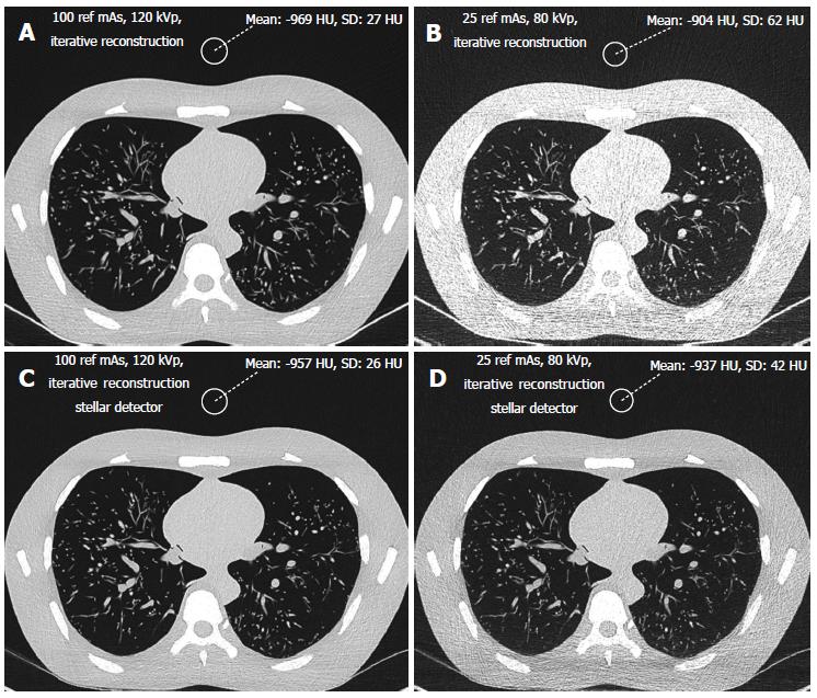
Engineering progress has greatly reduced the radiation dose required for computer tomography. Dose modulation along the x-, y- and z-axes[1-6] and shielding[7-12] represent major manufacturing steps involved in radiation protection. Increasing computing capacity has allowed iterative reconstruction to be introduced in the clinical routine, leading to dose reductions between 27% and 65%[13-18]. Problems with electronic noise during image acquisition can be overcome by integrating analog-digital-converters with the photodiodes on the CT-detectors contained on the same silicon chip (Stellar detector, Siemens Healthcare, Erlangen, Germany) with the potential to further reduce radiation dose[19].
Image quality can be characterized by calculating the noise, signal to noise ratio (SNR) and contrast to noise ratio (CNR)[20-24]. The signal at a region of interest (ROI) corresponds to the attenuation in Hounsfield units (HU). The noise corresponds to the standard deviation of the pixel attenuation within the ROI[20]. The signal will remain the same with lower tube current and unchanged tube voltage, but the noise will increase[21]. Several studies have demonstrated the feasibility of low dose imaging using a lowest acceptable tube current below 50 mAs for lung nodule detection[25-28].
Changing tube voltage changes the signal and the noise, depending on the absorption spectrum of the scanned object[21]. The dose (D) is coupled with many variables: D~(signal to noise)2/(pixel-size*image-thickness), D~mAs (Miliamperesecond) and D~kVp2 (Kilovolt peak)[20,21,25]. Noise reduction can either be used for dose reduction or to increase the image quality.
It is not known if the same CT dose is required to generate the same CNR with the new generation of CT scanners. Therefore, we investigated how the lowest acceptable signal to noise acquired at 50 mAs/80 kVp and used for filtered back projection can be transferred to iteratively reconstructed images using a new detector. We compared the dependency of dose and noise (SNR and CNR) for the last three generations of CT scanners.
A lung phantom (Chest Phantom N1 by Kyoto Kagaku) was used in this study (Figure 1). This phantom is an accurate life-size anatomical model of a male human torso with a synthetic heart, trachea, pulmonary vessels (right and left) and abdomen (diaphragm) block. The thickness of the chest wall is based on measurement of clinical data. The soft tissue substitute material (polyurethane, gravity 1.06) and synthetic bones (epoxy resin) have X-ray absorption rates very close to those of human tissues. The abducted arm positions of the torso are appropriate for CT scanning. The pulmonary vessels are also spatially traceable.
The phantom size was 43 cm × 40 cm × 48 cm with a chest girth of 94 cm and a weight of 18 kg. The pleural cavity measured 268 mm (craniocaudal). The phantom was measured at the level of the lung apices using axial slices (140 mm × 400 mm) and at the level of the diaphragm (208 mm × 279 mm).
The phantom was scanned using 3 different CT scanners (Siemens SOMATOM Sensation, SOMATOM Definition Flash and SOMATOM Definition Edge, all from Siemens Healthcare, Erlangen, Germany). The scan parameters were identical to the manufacturer’s standard presetting for THORAX ROUTINE: 24 mm × 1.2 mm, pitch 0.8 mm and slice thickness 1.5 mm for the SOMATOM Sensation 64; 128 mm × 0.6 mm, pitch 0.6 and slice thickness 1 mm for the SOMATOM Definition Flash; and 128 mm × 0.6 mm, pitch 0.6 and slice thickness 1 mm for the SOMATOM Definition Edge. The scan length and field of view (FOV) were 35 cm and 33 cm, respectively. Nine different exposition levels were used (reference mAs/tube voltage): 100/120, 100/100, 100/80, 50/120, 50/100, 50/80, 25/120, 25/100 and 25 mAs/80 kV. The option CARE kV setting that automatically adjusts tube voltage to an optimal level was disabled so that we could set the voltage to the predefined values. Reference mAs were used to keep the study parameters as close as possible to those used for routine scans. Images from the SOMATOM Sensation 64 were reconstructed using the classic filtered back projection method with a soft tissue kernel of B20 and a lung kernel of B60. Iterative reconstruction (SAFIRE, level 3) was performed for the two other scanners using the I26f and I70f Kernels. The dose was represented by the dose length product DLP (mGycm) provided by the scanners for a 32 cm diameter phantom for each scan with a constant scan length of 35 cm.
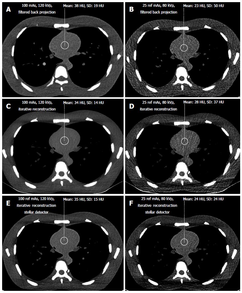
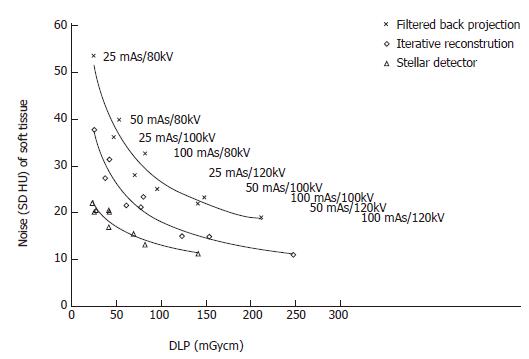
Signal and noise were recorded by two different radiologists with 10 and 3 years of experience, respectively, in chest CT radiology using a Picture Archiving and Communication System (PACS Philips Netherlands/Sectra Sweden). They measured the density in HU (signal) and the standard deviation of the CT values (noise) from regions of interest (ROIs) of 2 cm (3.14 cm2) in diameter. The ROIs were placed in air outside the phantom, anterior to the sternum (Figure 1) in bone (middle of the vertebral body) and soft tissue (heart, Figure 2). Each radiologist chose 5 different levels at which to place the ROIs in the phantom scans. Signal and noise were measured from the same ROIs. Measurements were recorded for air and bone using a hard Kernel and for soft tissue using a soft Kernel. The image quality (SNR) was calculated for soft tissue. Only the noise was recorded for air because the signal in air was negligible. Dose was represented by the dose length product DLP (mGycm) calculated automatically by the scanner for a 32 cm diameter phantom for each scan with a constant scan length of 35 cm. CNR was defined as the difference between the signal from the bone and the soft tissue divided by the noise: HUbone-HUsoft tissue/noise[29].
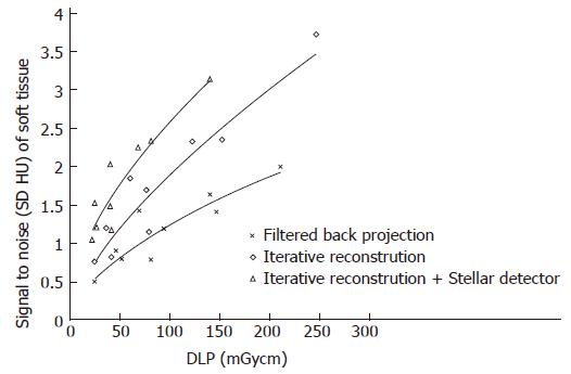
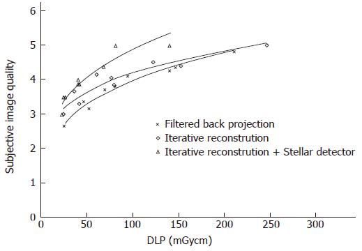
In addition, both radiologists scored the subjective image quality from 1 to 5 in the lung window (level -500 HU, width 1500 HU, Figure 1) using a hard Kernel on a Picture Archiving and Communication System (PACS Philips Netherlands/Sectra Sweden). The subjective image quality scale was as follows: (1) non-diagnostic; (2) poor, diagnostic confidence significantly reduced; (3) moderate, but sufficient for diagnosis; (4) good; and (5) excellent. Curves were fitted for the noise vs dose and for the SNR vs dose. The highest R-square correlation coefficients were observed for power curves. For the same noise or same SNR, this allows the corresponding CT acquisition dose for the different scanners to be exactly determined. The lowest acceptable doses of 50 mAs and 80 kVp determined from the filtered back projection method were transferred to image acquisition with iterative reconstruction with Stellar detectors.
To compare the different scans, it was necessary to transform the noise and the dose to obtain the same acquisition parameters as the SOMATOM Sensation. The dose and noise were therefore calculated for a standard slice thickness of 1.5 mm (SOMATOM Sensation). Because the dose remains constant when slice thickness is increased from 1 to 1.5 mm for the new generation Siemens scanners (SOMATOM Definition Flash and Edge), only the noise was corrected by a factor of 1/(1.5)(1/2)[22,23].
Graphs for image noise vs radiation dose and SNR vs dose were evaluated for air, soft tissue and bone. Trend lines were determined for the data points using regression to produce power curves in MedCalc® Version 7.6.0.0 and Microsoft Excel 2007. Noise reduction between two scanners was determined by subtracting the power curves. The integral of this subtraction equals the area between the curves. This area was divided by the dose to obtain the average noise reduction. The integral for the subtraction of the trend lines was calculated from the lowest (l) to the highest (h) joint radiation exposure according to
Math 1
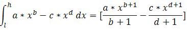
The dose reduction for a constant noise value was integrated along the noise scale to determine the average dose reduction. The smallest and highest reductions were determined to indicate the range. The Wilcoxon test for non-normally distributed paired samples was used to calculate the significance levels for noise reduction among the different scanners[30,31]. Inter-observer comparisons of the image quality score were performed, calculating the agreement levels with the Fleiss’ K statistic[32,33]. The K strengths were categorized as follows: < 0.20 poor, 0.21-0.40 fair, 0.41-0.60 moderate, 0.61-0.80 good, and 0.81-1.00 very good[34]. The Wilcoxon test and the Fleiss’ K statistic were analyzed in MedCalc® Version 7.6.0.0.
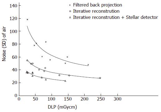
The noise levels measured in air, soft tissue and bone were significantly lower for iterative reconstruction compared to filtered back projection (P < 0.0001) and for using Stellar detectors in combination with IR compared to IR alone (P < 0.0001). The inter-observer agreement on image quality was moderate (kappa = 0.508). Noise/dose signature graphs for each scanner were plotted for air and soft tissue (Figures 3-5).
Noise reduction: The average noise reduction from filtered back projection (FBP, SOMATOM Sensation) and iterative reconstruction (IR, Somatom Definition Flash) was 10 HU (7-15 HU) for the same radiation dose, generating 31% (30%-31%) less noise. Changing from IR to the Stellar detector (Sd, SOMATOM edge) allowed another 7 HU (4-16 HU) of noise to be removed. Noise was reduced on average by (32%); 24% for the highest dose and 42% for the lowest dose (Figure 3 and Table 1).
Dose reduction: For a constant noise level, the dose could be reduced by an average of 53 (25-116) mGycm by applying IR instead of FBP, corresponding to an average dose reduction of 52%. At the lowest dose (high noise level), the dose reduction was 50%. At the highest dose, the dose reduction was 55%. An additional 69 (46-96) mGycm reduction was possible using the Stellar detector (54%). More dose reduction was achieved for the highest noise level (65%) compared to the lowest noise level (39%, Table 1).
Signal to noise (SNR ranged from 0.5 to 3.7, Figure 4): When dose was held constant, the SNR could be increased on average to 0.7 (36%, ranging from 0.2 to 1) and 0.6 (38%, ranging from 0.5 to 0.8) using IR and IR/Stellar detectors, respectively. Using a constant SNR, the dose could be reduced on average by 59 mGycm (45%, ranging from 20 to 107 mGycm) and 52 mGycm (41%, ranging from 23 to 72 mGycm) for IR and IR/Sd, respectively (Figure 4 and Table 2).
Noise reduction: A noise range of 23 to 118 HU was
measured for all scans. Noise levels for Sd were always lower than for FBP, even when comparing the lowest dose of Sd against the highest dose of FBP (Figure 5). Noise at the same dose level could be lowered by 31 HU (44%) and 12 HU (31%) on average by changing from FBP to IR and from IR to Sd, respectively. The largest noise reductions were possible at lower dose levels (Figure 5, Table 1).
Dose reduction: To maintain a constant noise level, the dose was reduced by 133 (106-165) mGycm and 106 (65-166) mGycm when using IR instead of FBP and Sd instead of IR only, averaging dose reductions of 80% and 70%, respectively. The relative dose reductions were higher at higher noise levels (Figure 5, Table 1).
Bone: The noise ranged from 80 to 382 HU. The average noise reductions at constant radiation levels were 64 HU (30%) and 24 HU (15%) using IR and Sd, respectively. At higher dose levels, there was less noise reduction (Table 1). For a constant noise level, the doses could be lowered by 48 mGycm (30%) and 35 mGycm (27%) on average for IR and Sd, respectively. The dose reduction was higher at higher noise levels (Table 1).
Contrast to noise: With the same radiation dose, an average of 34% (22%-37%) and 25% (13%-46%) greater CNR was achieved by changing from FBP to IR and from IR to Sd, respectively. For the same CNR, the dose could be reduced on average by 59% (46%-71%) and 51% (38%-68%) for IR and Sd, respectively.
Subjective image quality (5 points maximal, Table 2): Image quality rose by 0.2 (0.1-0.4) points and 0.5 (0.2-0.9) points on average by changing from FBP to IR and from IR to Sd, respectively (Figure 6). For the same image quality, dose could be reduced by 25% (2%-42%) and 44% (33%-54%) using IR and Sd, respectively (Table 2).
By setting the image quality along with the noise, SNR and CNR, our study showed that iterative reconstruction and Stellar detectors produce better quality images than scans reconstructed with filtered back projection using lower CT doses. Using the SOMATOM Definition Flash instead of the Sensation enabled either a dose reduction of 80% or a noise reduction of 44% when imaging air. It is not possible to achieve simultaneous dose and noise reduction. Additionally, at the level of maximal dose reduction, it is not possible to further increase image quality and vice versa. It is known that iterative reconstruction approaches (Adaptive Statistical Iterative Reconstruction or Sinogram Affirmed Iterative Reconstruction) can in some cases reduce radiation dose by 27% to 65%[13-18]. Our phantom study results confirm these findings, showing dose reductions of 30%, 52% and 80% for imaging bone, soft tissue and air, respectively.
Using the recently introduced Stellar detector, signal-transformation was implemented into the detector itself to reduce electronic noise. With this technique, it was possible to further reduce radiation dose by an average 27%, 54% and 70% for bone, soft tissue and air, respectively.
With lower tube voltage, not only did the image noise increase, but the density of the bone also increased, which is well known for dual energy scans. When the signal increased, the SNR also increased, altering the bone diagram. This is most likely the main reason why the Stellar detectors did not have the same effect on dose reduction when imaging bone. The benefit of dose reduction is greater for low doses, especially for bone and air. The absolute dose reduction, measured in mGycm, was larger at high doses, but the relative reduction was always larger at lower doses. This was true with the exceptions of subjective image quality and SNR, which are influenced by increased signal at lower doses (such as the case of bone). The manufacturer claims that Stellar detectors reduce noise by 20%[19]. However, because dose increases by a power of 2 as noise decreases, a potential dose reduction of 36% should be possible. We produced dose reductions of 27%-70% and noise reductions of 15%-32%. As mentioned above, the lower the dose levels, the bigger the relative benefit. Our scan range covered only low dose levels, with a high dose of 250 mGycm (100 reference mAs/120 kVp), equivalent to approximately 3 mSv. At high dose levels, the noise reduction approached 20% (24%, 28% and 7% for air, soft tissue and bone, respectively). The noise level was strongly influenced by the chosen kernel. For FBP reconstruction, there was a tradeoff between spatial resolution and noise. This tradeoff could be adjusted by selecting different kernels. Soft tissue kernels had much lower standard deviations in the signal than hard kernels for air and bone. Therefore, it was necessary to use the same kernels for comparisons. Some radiation protectors believe that the risk from high radiation (atomic bombs) can be extrapolated to much lower radiation exposures (CT) and that the risk of death due to radiation-induced cancer for the general population is 0.005%/mSv[35]. The conversion coefficient from DLP to mSv is 0.014 for lung[36,37], equivalent to a reduction of radiation induced cancer death per chest CT from 1 in 13000 for iterative reconstruction to 1 in 32000 when using Stellar detectors. These estimates neglect the potential bio-positive effects of low radiation exposure[38-42]. Nevertheless, radiation is a cumulative physical quantity that may lead to stochastic processes such as carcinogenesis. Therefore, radiation protection is mandatory even at lower dose levels.
In a previous phantom study using the SOMATOM Sensation, it was shown that the sensitivity for lung nodule detection was not significantly altered for images acquired with 50 mAs and 80 kVp compared to 100 mAs and 120 kVp (article submitted). With the findings from our present study, it is possible to transfer these parameters to new scanners that use iterative reconstruction and better detectors. Our images had noise levels of 81 and 40 HU for air and mediastinum, respectively. For similar noise levels, parameters as low as 25 mAs and 80 kVp for the SOMATOM Definition Flash and Edge are theoretically sufficient for detection without loss of sensitivity (Figures 3-5).
Obviously, image quality is not only defined by signal but also by contrast and noise because a loss of subjective image quality is less impressive than an increase in noise level. In other words, radiologists rate image quality higher than the measured noise would suggest. Perception of image quality is influenced by spatial resolution, individual vision and pattern recognition, all of which cannot be precisely measured. Fortunately, subjective image quality was not rated below what the noise level would predict.
Noise is one parameter of image quality, but we did not investigate scan plane and z-axis spatial resolution (Z-sensitivity) or high-contrast resolution[22]. Further studies are needed to investigate these parameters to understand how the type of scanner can influence image quality. The pre-settings for THORAX ROUTINE were not the same for the three scanner types. For example, the pitch for the Sensation was 0.8, but this value was altered to 0.6 for the other scanners. Increasing the pitch from 0.6 to 0.8 did not change the noise; however, the dose decreased corresponding to a Siemens specific unchanged tube current time product/pitch[43]. Therefore, it is possible that the images acquired by the Somatom Sensation have slightly different dose levels at lower pitches. The resolution was slightly different for the B- and I-Kernels for the different reconstruction approaches, which might have negatively influenced the noise of the I-Kernel. Ongoing studies will address this topic.
As varying kVp lead to CT number changes, it can be difficult to interpret results, especially for SNR and CNR. Possible differences in gantry geometry, detector efficiency and tube spectrum for the three investigated scanners were also neglected because our intent was to give an approximation of dose and noise reduction among the last three generations of CT for given clinical presettings. Varying the kVp also provoked questions about how beam-hardening effects impact the images, which will require further investigation.
To evaluate the dose reduction provided by the new Stellar detector, it would be desirable to compare images reconstructed using the FBP algorithm, which is a linear algorithm with predictable performance. We only compared SAFIRE reconstructed images with and without the Stellar detector. Due to the nonlinearity of iterative reconstruction methods, reconstruction may be object and dose dependent. Thus, it is difficult to characterize the improvements provided by the Stellar detector alone from the results in our study. Further investigations need to address this topic.
In conclusion, this study demonstrated an average dose reduction of 27% to 70% by applying the new Stellar detector. This dose reduction was equivalent to using IR instead of FBP.
Due to increasing computing capacity, iterative image reconstruction can be introduced into clinics, leading to the potential for dose reduction by replacing older filtered back projection methods. The problem of electronic noise during image acquisition was overcome by integrating the analog-digital-converter with the photodiode of the computed tomography (CT)-detectors on the same silicon chip. This noise reduction can either be used for dose reduction or to increase the image quality. The three latest CT-scanner generations were examined to compare their potential for dose reduction.
Several studies demonstrated the feasibility of low dose imaging without loss of sensitivity for pulmonary diseases. Radiologists are able to lower the CT tube current and/or the tube voltage, using the lowest acceptable published dose levels for older CT scanners. Manufacturer dependent progress in CT-technology was only partly investigated. Dose or noise reduction using iterative reconstruction has been published, but the potential for new detectors in the clinic is not yet known.
This study demonstrates the dependency of CT radiation dose, image quality and CT-generation. It is possible to obtain the same image quality with a dose reduction of 30% to 80% by substituting filtered back projection with iterative image reconstruction. Using the new CT-detectors, radiation dose can be reduced by an additional 27% to 70%, depending on the scanned tissue.
With the results, the lowest acceptable tube currents and voltages for the older CT-generations can be transferred to the newest scanners.
CT-exams produce cross sectional images of the body, based on the radiation absorption of the body tissues. Radiation absorption is measured at every angle circularly around the body and is back-projected on a virtual pixel field in the scanned plane, delivering a filtered back projection image. New iterative reconstruction methods distribute the absorption of one angle to all of the pixels in a direction, adjusting the pixel values based on the effective absorption for each angle position. For clinical routines, three iterations of 360° rotation are used, which is very time-consuming. Only recently was it possible to deliver sufficient computing power for these clinical scanners.
This manuscript described an interest work that the average dose could be reduced 30%, 52% and 80% for imaging bone, soft tissue and air for the same image quality by using iterative reconstruction instead of filtered back projection. In addition, employing the new Stellar detector could further lower radiation dose additionally by 27%, 54% and 70% for bone, soft tissue and air, respectively. The manuscript can be accepted for publication as it is.
PMC
Luciane Almeida Amado Leon
1 Laboratory of Technological Development in Virology, Oswaldo Cruz Institute Foundation, Rio de Janeiro, RJ, Brazil,
Adilson José de Almeida
2 Laboratory of Viral Hepatitis, Oswaldo Cruz Institute Foundation, Rio de Janeiro, RJ, Brazil,
Vanessa Salete de Paula
1 Laboratory of Technological Development in Virology, Oswaldo Cruz Institute Foundation, Rio de Janeiro, RJ, Brazil,
Renata Santos Tourinho
1 Laboratory of Technological Development in Virology, Oswaldo Cruz Institute Foundation, Rio de Janeiro, RJ, Brazil,
Daniel Antunes Maciel Villela
3 Scientific Computing Program Department-PROCC, Oswaldo Cruz Institute Foundation, Rio de Janeiro, RJ, Brazil,
Ana Maria Coimbra Gaspar
1 Laboratory of Technological Development in Virology, Oswaldo Cruz Institute Foundation, Rio de Janeiro, RJ, Brazil,
Lia Laura Lewis-Ximenez
2 Laboratory of Viral Hepatitis, Oswaldo Cruz Institute Foundation, Rio de Janeiro, RJ, Brazil,
Marcelo Alves Pinto
1 Laboratory of Technological Development in Virology, Oswaldo Cruz Institute Foundation, Rio de Janeiro, RJ, Brazil,
Conceived and designed the experiments: LAAL MAP AMCG. Performed the experiments: RST LAAL VSP. Analyzed the data: AJA DAMV. Contributed reagents/materials/analysis tools: LLLX. Wrote the paper: LAAL VSP MAP.
Associated Data
- Supplementary Materials
- S1 File: Individual data of anti-HAV antibodies, ALT and HAV-RNA in serum and saliva, according the day of diagnosis (dpd). Age (years); IgM and total anti-HAV are shown as DO/CO; IgM anti-HAV DO/CO ≥ 1.0 were considered positive; Total anti-HAV DO/CO ≤ 1.2 were considered positive; ALT: alanine aminotransferase; Viral load (copies/mL); ND: Not detected.
(DOC)
GUID: 2B409DD1-9551-4124-8714-61C5AACE2BBC
- Data Availability Statement
All relevant data are within the paper and its Supporting Information file.
Abstract
Despite the increasing numbers of studies investigating hepatitis A diagnostic through saliva, the frequency and the pattern of hepatitis A virus (HAV) markers in this fluid still remains unknown. To address this issue, we carried on a longitudinal study to examine the kinetics of HAV markers in saliva, in comparison with serum samples. The present study followed-up ten patients with acute hepatitis A infection during 180 days post diagnosis (dpd). Total anti-HAV was detected in paired serum and saliva samples until the end of the follow-up, showing a peak titer at 90th. However, total anti-HAV level was higher in serum than in saliva samples. This HAV marker showed a probability of 100% to be detected in both serum and saliva during 180 dpd. The IgM anti-HAV could be detected in saliva up to 150 dpd, showing the highest frequency at 30th, when it was detected in all individuals. During the first month of HAV infection, this acute HAV marker showed a detection probability of 100% in paired samples. The detection of IgM anti-HAV in saliva was not dependent on its level in serum, HAV-RNA detection and/or viral load, since no association was found between IgM anti-HAV positivity in saliva and any of these parameter (p>0.05). Most of the patients (80%) were found to contain HAV-RNA in saliva, mainly at early acute phase (30th day). However, it was possible to demonstrate the HAV RNA presence in paired samples for more than 90 days, even after seroconversion. No significant relationship was observed between salivary HAV-RNA positivity and serum viral load, demonstrating that serum viral load is not predictive of HAV-RNA detection in saliva. Similar viral load was seen in paired samples (on average 104 copies/mL). These data demonstrate that the best diagnostic coverage can be achieved by salivary anti-HAV antibodies and HAV-RNA tests during 30–90 dpd. The long detection and high probability of specific-HAV antibodies positivity in saliva samples make the assessment of salivary antibodies a useful tool for diagnosis and epidemiological studies. The high frequency of HAV-RNA in saliva and the probability of detection of about 50%, during the first 30 dpd, demonstrate that saliva is also useful for molecular investigation of hepatitis A cases, mainly during the early course of infection. Therefore, the collection of saliva may provide a simple, cheap and non-invasive means of diagnosis, epidemiological surveys and monitoring of hepatitis A infection purposes.
Introduction
Hepatitis A virus (HAV) is the most common agent causing acute liver disease with approximately 1.4 million of new cases occurring every year worldwide [1]. It is a significant health problem in primary school due to the clinical aspect of the disease where asymptomatic patients contribute to disease spread among children, causing outbreaks that can be propagated to community. Studies have shown that in developing countries improvements in sanitary conditions have led to a reduction in childhood exposure to HAV, resulting in an increased disease burden in older population groups [2,3] and also several outbreaks [4,5].
Very sensitive and specific serological tests for detection of HAV antibodies are widely available for serum samples. They are key tools for diagnosis, epidemiological knowledge and prevention strategy whereby infected or susceptible persons can be identified, and directed to a medical care or vaccination program in order to prevent or reduce further transmission in these populations. However, many studies have shown that saliva have a great potential as alternative tool for diagnosis of several viral diseases, such as by human immunodeficiency virus (HIV) [6,7], hepatitis A [8,9,10], hepatitis B [11], hepatitis C [12,13], and herpes simplex [14].
The collection of saliva as an alternative to blood collection offers potential advantages for diagnosis and epidemiological studies. Due to its minimally invasive and simple collection, saliva testing can reduce discomfort, a major concern to children, thereby simplifying diagnosis and the collection of serial samples for monitoring disease states over time. Besides, it allows a noninvasive investigation of HAV subclinical cases, which occur frequently among children, and facilitates HAV vaccination candidates tracing. Thus, in recent years, has aroused a lot of interest in saliva as source of HAV antibodies and viral detection for diagnosis purposes and monitoring hepatitis A.
However, the concentration of IgG in saliva has been reported to be substantially lower (average 300 times) when compared to its concentration in serum [15,16,17]. Many studies have reported sensitivity and specificity rates comparable to those observed in blood-based tests [8,9,18,19], while others have demonstrated problems with assay sensitivity due to the low antibody levels in saliva [20]. Then the lower antibodies titers in saliva may become undetectable earlier than in serum.
Despite few reports evidenced the presence of HAV RNA in oral fluid [9,21], the frequency and load of HAV in it remains still controversial [22,23,24]. The knowledge of the true frequency of oral carriage of HAV and if the levels of the virus in oral fluids correlate with those of blood, may be central to suggest oral fluids as a vehicle of the transmission of hepatitis A and also to determine if saliva can be a tool to conduct molecular epidemiological studies of HAV.
These inconsistent data warrant the need for well-planned longitudinal studies to explore the precise frequency and pattern of anti-HAV antibodies and HAV-RNA in oral fluid in comparison with serum, in order to stablish if saliva may be useful for epidemiological studies, diagnosis and monitoring of hepatitis A. In particular, this approach is very important for intermediate endemic regions where HAV vaccination is critical to control the large outbreak of epidemics. Thus, the aim of this study was to describe the serological and virological course of hepatitis A infection through a longitudinal analysis of salivary antibodies and viral load pattern.
Material and Methods
Studied population
Patients attending to the Viral Hepatitis Ambulatory (VHA) of Institute Oswaldo Cruz, Rio de Janeiro, Brazil, during May 2009 to January 2010, with signs and/or symptoms of acute viral hepatitis such as jaundice, fever, general malaise, fatigue, nausea, vomiting, and anorexia, were screened for the study. After laboratory diagnosis of hepatitis A by detection of serum IgM anti-HAV antibodies, 10 patients were invited to participate into the longitudinal follow-up, where consecutive blood and saliva specimens were collected at 0, 30, 90, 120, 150, and 180 days post diagnosis (dpd). No sample was collected before the onset of illness. The ‘0th’day was defined as the day of hepatitis A diagnosis.
Ethical aspects
Ethical permission for collecting and testing samples was provided by the FIOCRUZ Ethical Committee (536/09). Before entering into the study, all subjects or their guardians, on behalf of the minors/children enrolled in the study, have signed a written informed consent, previously approved by the Fiocruz ethical committee. The specimens were anonymous feedback was given to all participants of the study, including their results.
Biological samples
All saliva samples were collected using OraSure collection devices (Epitope Incorporated, Beaverton, OR, USA) according to the manufacturer’s instructions. Samples were later recovered by centrifugation at 2500×g for 15 min at 10°C and stored at −20°C until analysis. Total blood samples were collected by venipuncture into sterile tubes, after which serum was obtained by centrifugation and stored at −20°C. Serum samples were conventionally used for serological and molecular diagnosis of HAV infection, and considered as the ‘gold standard’ for comparison with saliva tests [25].
Liver function
Laboratory determination of serum alanine aminotransferase (ALT) and aspartate aminotransferase (AST) levels were carried out by a manual colorimetric procedure using a commercially available kit (Abbott, North Chicago, IL, USA).
Detection of specific anti-HAV antibodies in serum and saliva
Serum IgM and total anti-HAV antibodies were detected by using enzyme immunoassays (Biokit, Barcelona, Spain) according to the manufacturer’s instructions. For saliva samples, undiluted samples (100 μL and 15 μL for IgM and total anti-HAV, respectively) were tested in a modified ELISA (Biokit, Barcelona, Spain) [9]. The cut-off point for HAV antibody detection was evaluated based on receiver operating characteristic curve (ROC curve) analysis (MedCalc for Windows, version 7.6.0.0, MedCalc Software, Mariakerke, Belgium). The ability of the model to differentiate between positive and negative individuals for total and IgM anti-HAV antibodies (discrimination) was quantified using the area under the curve (AUROC) test [26,27].
Detection and quantification of HAV-RNA in serum and saliva samples
HAV-RNA was extracted using the QIAamp™ viral RNA extraction kit (Qiagen, Germany). A TaqMan real-time PCR assay was performed to quantify HAV genomes as previously described by de Paula et al. [28]. Viral RNA was amplified using primers derived from the most conserved region of HAV genome, the 5’ non-coding region (5’ NCR). The cDNA synthesis was carried out using 10 μL of RNA (10 pg– 5 μg), 10 pmol/μL of anti-sense primer (HAV5NCRI-R), 1 U/μL of RNasin (Promega, Madison, WI), 125 mM of each deoxynucleoside triphosphate, and 1 U/μL of Superscript III (Invitrogen, Carlsbad, CA, USA), in a final volume of 20 μL at 50°C for 1 h, followed by incubation for 10 min at 65°C. After cDNA synthesis, a master mix containing 1x TaqMan Universal PCR Master Mix (Applied Biosystems, Hammonton, NJ, USA) and 1.25 μL of the assay mixture (300 nM each primer, 150 nM probe) (Applied Biosystems Assay, Foster City, CA, USA) was prepared. Five microliters of cDNA and standard curve points were added to 20 μL of the PCR master mix. The thermal cycling conditions were as follows: an initial step at 50°C for 2 min and 95°C for 10 min, followed by 40 cycles at 95°C for 15 s and at 60°C for 1 min. The primers and probe used to quantify the 5′NTR are described by de Paula et al. [28].
Statistical Analysis
We used Chi-square test and student’s t-test as appropriate. The Mann–Whitney U-test was used to evaluate differences between continuous variables (age and viral load). The diagnostic value of anti-HAV antibodies assay in saliva samples was assessed by receiver operating characteristic (ROC) curve. An area under curve (AUC) of 1.0 is characteristics of an ideal test, whereas 0.5 indicates a test of no diagnostic value. All data were analyzed by two tailed tests and a p value less than 0.05 was considered significant.
The kinetics of total and IgM anti-HAV titers, and viral load were analyzed as separate univariate models by applying Generalized Additive Model with Mixed effects (GAMM), where the time after illness onset was considered as explanatory variable using a smoothing spline and random effects per patient, with Gaussian error distribution and identity link function. After fitting models we found mean values and 95% confidence intervals to describe kinetics for both saliva and serum samples. In order to estimate probabilities of test positivity at days after illness onset for each of the diagnostic outcomes (total anti-HAV titre, IgM anti-HAV titre, and viral load), we take the binary outcomes (positive/negative) from each of the test results and their counts were used as observations for fitting logistic regression models. Number of days after illness onset and sample type (saliva/serum) are explanatory variables and a log link function is used. Analyzes were performed using R software [29] and package GAMM4 [30].
Results
Demographic characteristics of studied population
Ten patients with acute hepatitis A, aged 3–28 years (14.3 ± 7.6 years), five of them were males, was included in this study. All participants were followed up to 180 days, except for patient 10 (p10) who was followed up until 120 days.
Anti-HAV antibodies response and biochemical profile during the follow-up of HAV cases
In Fig 1, the individual analysis of HAV antibodies profile in paired serum and saliva samples, and serum ALT levels are presented for all patients (p1 –p10), during the follow-up period. In all individuals, ALT levels were elevated during the first 30 days, but declined to baselines values afterwards. The outcome for total anti-HAV tests was positive for all individuals in both saliva and serum up to the end of the study. However, in most of the patients (7/10) total anti-HAV OD/CO was higher in serum than in saliva samples during the course of infection.

Age (years); *IgM and total anti-HAV are shown as DO/CO; IgM anti-HAV DO/CO ≥ 1.0 were considered positive; Total anti-HAV DO/CO ≤ 1.2 were considered positive; # HAV-RNA detection are shown as + (positive) or—(negative); ** Patient 10 (p10) was followed up only until 120 days.
The IgM anti-HAV was detected in saliva of all individuals at 30th and patients were likely to remain IgM positive in paired serum and saliva samples, up to day 120. However, in five individuals (p1, p4, p5, p6 and p7), salivary anti-HAV IgM remained detectable for longer than in serum samples (Fig 1) (S1 File).
Fig 2 shows the overall kinetics of serum and saliva IgM and total specific-antibodies and the probability of these markers detection along the course of infection. IgM and total anti-HAV was detected already on the 30th, the earliest serum and saliva samples. The kinetics of total anti-HAV in saliva showed a peak of the titer on the 90th, followed by a decreasing trend of the titers afterwards. While in serum samples, total anti-HAV titer tend to increase until the end of the follow-up, and in general, this titer was higher in serum than in saliva samples (Fig 2A). This HAV marker showed a probability of 100% to be detected in both serum and saliva during 180 dpd (Fig 2B).

Solid lines and shaded areas along them represent for saliva the predicted mean values and 95% confidence intervals, whereas dashed lines and respective shaded areas represent for serum results the predicted mean values and 95% confidence intervals. In A-C-E, circles and triangles represent individual observations for saliva and serum, respectively, and in B-D-F, represent the counts of positive tests (value 1) or negative (value 0) for saliva and serum, respectively. Shape sizes (circles and triangles) are proportional to the counts.
Along the course of infection, IgM anti-HAV demonstrated a similar pattern of response in paired specimens. During the first month of HAV infection, this acute HAV marker showed a detection probability of 100% in paired samples. On the 90th, 80% of the saliva and serum samples were still positive for IgM anti-HAV, with a probability of 85% (95% CI: 70–100%) and 74% (95% CI: 50–96%) for IgM anti-HAV detection in saliva and serum, respectively. Overall, patients were likely to remain IgM positive in paired serum and saliva samples, up to illness day 120, with a probability of 24% (95% CI: 4–43%) and 39% (95% CI: 16–62%), respectively (Fig 2D).
No significant difference was observed between serum and saliva IgM anti-HAV OD/CO (median = 1.88 in serum, and 1.87 in saliva) (p = 0.28) (Fig 2C). To determine a relative correlation between the level of IgM anti-HAV in saliva and its level in serum during the follow up, a statistical approach was used. From days 30–90 post onset, there was a high positive correlation between the optical density (OD) values in serum and saliva (r = 0.997 [95% CI = 0.97–0.99] p < 0.001). While, from days 120–180, a lower correlation was seen (r = 0.74 [95% CI = 0.29–0.92] p < 0.0056).
The association of IgM anti-HAV detection in saliva samples was evaluated with IgM antibody level [DO/CO] in serum, HAV-RNA detection and viral load in serum and saliva. Each parameter was grouped in two categories: IgM level (DO/CO): ≤ 5.0 and >5.0; HAV-RNA detection: positive and negative; viral load: ≥ 20.000 and < 20.000. No association was found between IgM anti-HAV positivity in saliva and any parameter (Fisher test, p>0.05 for each comparison).
Comparison of HAV-RNA detection and viral load between serum and saliva samples
In order to determine the duration of HAV detection and viral load in saliva, serial paired serum and saliva samples from 10 HAV patients were evaluated. HAV-RNA was more frequently detected during the early course of infection (at 30th) in serum (8/10) and in saliva (6/10) samples (Fig 1). An intermittent pattern of HAV RNA detection was seen in some individuals both in serum (p1, p2, p4, p6 and p8) and in saliva (p2 and p8) samples. Most of the patients positive for HAV RNA in saliva (8/10) also showed viremia. However, two patients (p4 and p5) were negative for HAV-RNA in saliva during all the follow up, and showed viremia. A delayed HAV-RNA detection was seen in patients p7 and p8 (from 180 and 120 dpd, respectively), in both kind of specimens, persisting detectable up to the end of follow-up (Fig 1). The mean viral load ranged from 103 to 105 copies/mL, in paired samples (Table 1) (S1 File), reaching a peak at the 30th, followed by a decreasing trend up to the end of follow up (Fig 2E).
Table 1
| patient | Time points (dpd) | |||||||||
|---|---|---|---|---|---|---|---|---|---|---|
| 30 | 90 | 120 | 150 | 180 | ||||||
| serum | saliva | serum | saliva | serum | saliva | serum | saliva | serum | saliva | |
| p1 | 8.4x10³ | ND | ND | ND | ND | 3.5x10⁴ | 3.0x10³ | 5.1x10⁴ | ND | ND |
| p2 | 1.5x10⁴ | 5.3x10⁵ | ND | ND | 2.6x10⁴ | 8.8x10³ | ND | ND | ND | ND |
| p3 | 4.3x10⁴ | 9.8x10³ | 4.4x10³ | 8.9x10³ | 3.6x10³ | 3.3x10³ | ND | ND | ND | ND |
| p4 | 3.6x10⁴ | ND | ND | ND | 2.6x10⁴ | ND | ND | ND | 1.9x10⁴ | ND |
| p5 | 9.3x10⁴ | ND | ND | ND | ND | ND | ND | ND | ND | ND |
| p6 | 2.8x10³ | 3.9x10³ | ND | ND | ND | ND | ND | ND | 1.3x10⁴ | ND |
| p7 | ND | ND | ND | ND | ND | ND | ND | ND | 1.9x10⁴ | 3.5x10³ |
| p8 | ND | ND | ND | ND | 1.2x10⁴ | 2.4x10⁴ | ND | ND | 9.0x10⁴ | 2.2x10³ |
| p9 | 5.8x10⁵ | 4.2x10⁵ | 1.9x10⁵ | 2.2x10⁴ | 7.1x10⁴ | 2.7x10⁵ | ND | ND | ND | ND |
| p10 | 1.2x10⁵ | 2.3x10⁵ | ND | ND | ND | ND | ND | ND | ND | ND |
| Mean (SD) | 1.1x10⁵ (1.9x10⁵) | 2.0x10⁵ (2.5x10⁵) | 7.1x10⁴ (9.2x10⁴) | 1.5x10⁴ (1.0x10⁴) | 3.1x10⁴ (2.8x10⁴) | 6.8x10⁴ (1.2x10⁵) | 3.0x10³ | 5.1x10⁴ | 4.0x10⁴ (4.2x10⁴) | 2.2x10⁴ |
| Total positive cases | 8/10 | 6/10 | 3/10 | 2/10 | 4/10 | 5/10 | 1/10 | 1/10 | 3/10 | 1/10 |
During the follow up, HAV RNA was detected in saliva with a probability ranging from 50% (95% CI: 28–72%) (at 30th) to 18% (95% CI: 4–31%), at the end of the study. While the probability to detect viremia ranged from 62% (at 30th) (95% CI: 41–83% to 26% at the end of the study (95% CI: 10–42%) (Fig 2F).
To clarify whether the detection of HAV-RNA in saliva is dependent on the patients’ characteristics, i.e. antibodies levels, ALT and AST levels, HAV-RNA detection and/or viral load, the association of HAV-RNA positivity in saliva samples was evaluated with patients’ characteristics (gender, age, ALT level, IgM antibody level [CO/DO], serum HAV-RNA detection, and serum and saliva viral load). Each parameter were grouped in two categories: gender: F and M; age (years): ≤ 5 and > 5; ALT level (U/L): 40–1000 and >1000; IgM level (CO/DO): ≤ 5.0 and > 5.0; serum detection: + and -; serum viral load (copies/mL): ≤ 20.000 and > 20.000; saliva viral load (copies/mL): ≤ 20.000 and > 20.000. No association was found between HAV-RNA positivity in saliva and any patient characteristic (Fisher test, p>0.05 for each comparison).
Discussion
Owing to the lower concentration of saliva IgM and IgG, and the controversial data about HAV-RNA detection in saliva, it is important to know the frequency and length of these HAV markers in the saliva samples to determine the feasibility and applicability of this fluid for diagnosis and epidemiological studies. Our previous studies demonstrated the detection of HAV specific-antibodies and HAV-RNA in saliva samples [9,31] of acute HAV cases. This further study is to the best of our knowledge, the first study to monitor the patterns of saliva immune response and genome detection during the course of hepatitis A infection, aiming to stablish if the saliva may be an alternative tool for the diagnosis, monitoring and epidemiological study of hepatitis A.
Although oral fluid collection has many advantages, when compared with total blood collection by venipuncture, some problems may arise if the choice of assay is not appropriate to detect antibodies in saliva samples. In the present study, an optimized assay was used to obtain optimal conditions for the detection of IgM and IgG anti-HAV antibodies in oral fluid [9]. In addition, a reduction of cut off value by approximately 18% was established, based on ROC curve analysis, to improve the test accuracy. The importance of establishing a cut-off ratio for the detection of HAV antibodies in oral fluid specimens has been demonstrated to be essential to increase the test accuracy [10].
During the course of HAV infection, it was demonstrated that total anti-HAV could be detectable in all patients, for at least 180 days after illness onset. However, a decreasing trend of the salivary total anti-HAV titer after 180th, suggests that, unlike the serum, it can become undetectable in saliva samples subsequently. The total anti-HAV DO/CO values were significantly lower in saliva, which confirms the lower titers of HAV antibodies in saliva [17]. This HAV marker showed a detection probability of 100%, until the end of the study. The long detection and high probability of total anti-HAV positivity in saliva samples make the assessment of salivary total anti-HAV a useful tool for diagnosis and epidemiological studies.
The profile of IgM anti-HAV response were quite similar between paired serum and saliva samples. However, in five individuals, salivary anti-HAV IgM remained detectable for longer that in serum samples. The longer detection of salivary anti-HAV IgM in these patients than in serum could be a reflects of a higher viraemia in serum samples, which may results in large amounts of IgM anti-HAV complexed with viral particles, becoming undetectable by serological assays. The difference of anti-HAV antibodies detection observed between patients was probably due the different phase of infection. Since the samples were collected from the day of hepatitis A diagnosis (‘0th’ day), the following days of collection did not represent a precise day of the infection. IgM anti-HAV could be detected in both types of samples from all subjects, on average, until 90 (ranging from 0 to 150) dpd. This finding is in accordance with a follow-up study conducted in 29 acute-phase patients that indicated that IgM anti-HAV persisted for 2–4 months and were not usually detectable thereafter [32].
Considering the good correlation (r = 0.99, p< 0.001) between the optical density (OD) values of the paired samples, the high frequency (100%-80%) and probability (100%-85%) of IgM anti-HAV detection in saliva of HAV acute cases at 30 and 90th (100%-80%, respectively); the salivary IgM anti-HAV test showed a potential of substitute serum test in diagnosis of hepatitis A infection, mainly during the first 90 days post infection. No association was seen between HAV antibodies detection in saliva and antibodies level in serum, or the HAV RNA detection and/or viral load, indicating that the detection of anti-HAV antibodies in saliva is not dependent on these parameters.
Most of the hepatitis A patients (80%) were found to contain HAV RNA in saliva, as reported earlier [9,21,33]. HAV-RNA was often detected at early acute phase (during the first 30 days) of the infection in serum and saliva samples. However, it was possible to demonstrate the viral persistence in paired samples for more than 90 days, even after seroconversion. These current findings revealed a longer saliva and serum viremia than that reported by Costa-Mattioli et al. [34] who demonstrated persistent viremia, for an average of 60 days after clinical onset. The different period of HAV-RNA detection among patients must reflect the different stages of infection, since in some patients HAV-RNA was eliminated early (after 30 days) and in others it could be detected lately (as of 150 days). However, some authors suggested that the duration of viremia is dependent on the immunological and/or biochemical profile of the host [35]. In the present study, considering that, during some time points of the infection, HAV viral load was higher in saliva from some patients than in serum, and no significant relationship was observed between salivary HAV-RNA positivity and serum viral load (p = 0.4 95% IC = 0.33–1.0), these findings show that viral load in serum is not a predictive factor of HAV-RNA detection in saliva, as has been reported early by Amado et al. [9]. A previous study suggested that the HAV viral load in saliva might reflect a local site of HAV replication, as has been demonstrated a HAV replication in salivary gland of experimentally infected cynomolgus monkeys [31]. Therefore, an active HAV replication in the salivary glands would perhaps explain the discrepant HAV detection between matched serum and saliva specimens observed on day 120, when there were more positive cases in saliva than in serum.
Based on our results, similar viral load levels were seen in paired serum and saliva samples from each patient (on average 104 copies/mL). Previous human HAV infections investigations have showed a mean serum viral load of 103 copies/ml [34,36]. The 2-log difference between serum and saliva samples reported by Mackiewicz et al. [21] was not observed in the present study, which could be probably attributed to the use of different methods of quantification and different timing of sample collection [37]. The kinetics of HAV-RNA detection in both serum and saliva showed an intermittent pattern of detection in some patients, probably due the fluctuation in the viral load, which has also been demonstrated by Amado et al. [31] in cynomolgus monkeys experimentally infected with HAV.
Taken together, the high frequency of HAV-RNA in saliva and the probability of detection of about 50%, during the first 30 dpd, demonstrate that saliva is useful for molecular investigation of hepatitis A cases, mainly during the early course of infection. Nonetheless, the intermittent pattern of detection and low probability of HAV-RNA detection, in paired samples, after the first month of infection, suggests that HAV-RNA detection is not a sufficient diagnostic tool for the whole time period. The relationship between HAV detection and infectivity has not been established yet and, in order to evaluate the potential risk of transmitting HAV by saliva among patients during early acute phase or convalescence period, it would be interesting to conduct experimental infection studies in animal models [34,38].
In summary, these data demonstrate that saliva samples could be used as a method of detecting anti-HAV antibodies and HAV genome, and that the best diagnostic coverage can be achieved by salivary IgM and total antibodies detection during the first 90 dpd, which quite correlates with serum methods. Therefore, the collection of saliva may provide a simple, inexpensive and non-invasive means of diagnosis, epidemiological studies and monitoring of hepatitis A infection purposes.
Supporting Information
S1 File
Individual data of anti-HAV antibodies, ALT and HAV-RNA in serum and saliva, according the day of diagnosis (dpd).Age (years); IgM and total anti-HAV are shown as DO/CO; IgM anti-HAV DO/CO ≥ 1.0 were considered positive; Total anti-HAV DO/CO ≤ 1.2 were considered positive; ALT: alanine aminotransferase; Viral load (copies/mL); ND: Not detected.
(DOC)
Funding Statement
Support was provided by the Fundação de Amparo a pesquisa do Estado do Rio de Janeiro [www.faperj.br], grant number: E-26/112.097/2013 to author: LAAL.
Data Availability
All relevant data are within the paper and its Supporting Information file.
References
What’s New in the MedCalc 7.6.0.0 serial key or number?
Screen Shot

System Requirements for MedCalc 7.6.0.0 serial key or number
- First, download the MedCalc 7.6.0.0 serial key or number
-
You can download its setup from given links:

MedCalc 7.6.0.0 serial key or number & for Laptop

MedCalc 7.6.0.0 serial key or number& for Laptop